Another Another New Tone Circuit (I think the last)

Introduction
I am very excite! I finally have the solution to my tone circuit. It's been a long time, and a lot work. I've been pretty happy with my improvement in intuition when it comes to analog circuits. These are very simple, but it's amazing what you don't know after leaving undergrad. It's fun to get to know subjects like this. Anyway, let's talk about the new (final) circuit.

Why the Change?
You may realize that I just posted a new circuit with the same capabilities (i.e. adjustment of cutoff frequency and adjustment of attenuation floor). This was the last post, and the circuit was completely passive. I did put the circuit together, and it sounded like it worked, but there was an additional problem that I did not foresee.

If you think about it, if we're adjusting both the real value of the impedance in the shunt portion of the low pass filter and the feed portion, we are going to change the DC gain. And this is exactly what happened to me. There was a dramatic drop in volume as I changed the cutoff frequency. I'm sure it was the case that the cutoff frequency did in fact change, but the drop in volume was unacceptable.

Avoiding the Volume Change
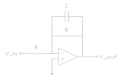
The thought occurred to me that an active filter might be able to compensate for the tendency of the circuit's DC gain to change with cutoff frequency. So I conceived the following circuit.

If you've read my previous post about a standard active 1-pole low pass filter, you should find this schematic familiar. I had implemented the circuit without R3 before, but I decided that the absence of an attenuation floor adjustment was too different than the original tone circuit. But I realized that you can add the floor feature by adding R3 to the circuit. Notice that all the pots in the circuit are wired as variable resistors (3rd terminal floating). In my implementation, R1=R2 to maintain unity gain.

Here's an intuitive description of the circuit. Recall that the standard opamp inverter has a gain of -R2/R1 where R2 is the feedback resistor and R1 is the input resistor. This still applies, but now R2 is replaced by a feedback network with complex impedance.

First ignore R3 (let's say that it's turned all the way down). We're back to the original filter. For high frequencies, the capacitor becomes a short, and the feedback impedance is 0 (so the gain is 0). For low frequencies, the capacitor is an open circuit, so the feedback impedance is simply R2.

Now let's consider R3. At high frequencies, the capacitor will still be a short circuit, but the feedback network's impedance will now be R2//R3 (which is less than R2). So we will still attenuate high frequencies, but R2//R3 is still a lot more than 0. R3 provides a floor for the attenuation. At low frequencies, the capacitor becomes an open circuit and R3 has no effect on the circuit. We're back to an impedance of R2, just like before we added R3.

Adjusting the cutoff frequency is as simple as adjusting R1 and R2. If we maintain the condition that R1=R2, then the DC gain will always be unity. So let's use a dual ganged pot. Radd is there to make sure we can't adjust the resistances in the circuit all the way down to 0. A value of 100 still yields roughly 7kHz for a maximum cutoff frequency.

The values I used in testing were as follows:
R1 = R2 = 5K Log Pot
R3 = 500 K Log Pot
C = 0.22uF
Radd = 100

Performance
Here is the plot of the frequency response. Again, I have used an animated GIF to show different values for R1 and R2. Each graph should resemble the original tone circuit response that came in the guitar. However, R1 and R2 give us the ability to adjust the cutoff frequency, whereas it is constant in the original tone circuit. And again, you can see that the DC gain of the circuit remains 1 (0dB) regardless of cutoff frequency.

** hmm i can't get this gif to work. I wonder if blogspot has changed their picture policy. I got a GIF up here before without any trouble. I guess you'll have to take my word for it for now.**

A Couple of Considerations
As I mentioned briefly, we can't have 0 ohm resistors in the feedback or input paths. This is the reason for Radd. Radd puts an upper limit on our cutoff frequency as well.

If our goal is to allow R3 to completely nullify the effects of the capacitor in the circuit when turned all the way up, then R3 needs to be much larger than R2. The value of R2 changes (obviously, that's the point), so often it will be small in the first place. The worst case is when we turn R2 all the way up (moving the cutoff frequency as low as it will go). At that point, putting R3 in parallel with R2 can affect the maximum attenuation floor realizable by the system. So even though the problem would be less evident at higher cutoff frequencies, the ability to nullify the capacitor would worsen as we adjusted down. Therefore, it is important to make R3 >> R2.

Of course, the price we pay for this adjustment is less precision on the R3 adjustment. However, as it turns out, R2 should only be 5K, so the original tone pot 500K will work nicely. I just ran the numbers for 250K, 100K, and 50K. At the lowest cutoff frequency, 250K looks good in the passband (a drop of less than .2 dB), but 100K and 50K have passband gains of more like -.5dB and -.8dB. That would probably be noticeable. But you'd have to listen to it.

Cutoff Frequency Selection
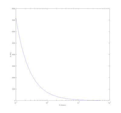
I graphed the cutoff frequency for 400 logarithmically spaced combinations of R1,R2 and R3 (20 values each). Here are the results.

The different traces are for different values of R3. As you can see, adjusting R3 has little effect on the cutoff frequency of the circuit. It does have a little more effect at higher cutoff frequency settings, but I don't think it's anything to be worried about. There are a couple of outliers, but this is probably a numerical artifact when R3 is set so that the attenuation floor is above -3dB. Obviously cutoff frequency has no meaning in this case, since it is defined as the frequency at which the circuit's gain is -3dB.

Calculating the Cutoff Frequency
One thing to mention is that the cutoff frequency is not as easy to calculate for this more complicated circuit as it is for the simple Active 1-pole filter. I worked out the math for a while, but it was clear that an analytical solution to the equation would be very difficult to obtain. So I had to solve for it numerically. I used the secant method, similar to Newton's Method, but without a requirement for the derivative of the function in question. I fixed the values for all the circuit's components, constraining the equation to one free variable. The code is included below.

Conclusion
I have put this together on a breadboard, and the results are excellent. Here are a couple of pictures of my setup. I just finished making that desk a couple of weeks ago. (designed in 3d autocad and put together with pocket hole screws). This is the first project on the new project desk. Yes I know the top is particle board. It is meant to be a project desk, not a piece of fine furniture.

I didn't have a dual ganged pot for the 5K, so I used 2 single ganged and one of my wife's thousands of hair rubber bands as a pulley belt. Not the best in the world, but it worked well enough for testing. I'm digging having the new desk. It's 72" by 26". Designed to fit in that space.

I'm very excited about finally solving this problem. Now I need to get a microcontroller and program the rest of the circuit. That will be another blog post to reveal why I need a microcontroller. Basically, I'm going digital on the blending pots.

Code
Here's the main simulation code.

% my adjustable tone control simulation
% This is an active circuit with a parallel combination of 
% R2 and (R3 in series with C1) in the feedback path.
% The input has R1 in series.  R1=R2 and they are variable.
% R3 is also variable.  C1 is constant.
% Normal Gain Equation is G = -R2/R1

% 0.22 uF capacitor
Ctone = 0.22e-6;

% Added Series Resistor to R1,R2
Radd = 100;

% Series Resistor with C1.  Affects the floor of the filter
R3Val = 500e3;
% steps on the tone resistor
R3 = logspace(0, log10(R3Val));

% Parallel Resistor and Input Resistor.  Affect the cutoff frequency of the filter
R1a2Val = 5e3;
% steps on the series tone resistor
R1a2 = logspace(0,log10(R1a2Val)) + Radd;

% steps in frequency
freq = logspace(0, log10(20e3), 100);

% Impedance of C1
ZCtone = repmat( (-j./(2*pi*Ctone*freq))' , 1, size(R3,2) );

% Resize R3
R3 = repmat(R3, size(ZCtone, 1) , 1);

% Series Impedance of Feedback Path 1
% Down = Frequency
% Across = R3 Changes
% Depth = R1 and R2 Change
Z1 = repmat( R3 + ZCtone, [1 1 size(R1a2,2)] );

% Resize R1a2 for operations with Z1
R1a2 = reshape( R1a2, [1 1 size(Z1,3)]);
R1a2 = repmat(R1a2, [size(Z1,1) size(Z1,2), 1]);

% Calculate Impedance of entire feedback path
Z2 = ( R1a2 .* Z1 ) ./ ( R1a2 + Z1 );

% Calculate the Gain
gain = abs(-Z2 ./ R1a2 );

% Calculate Cutoff Frequency
% Analytical solution is difficult, so let's use numerical methods
% below is the equation for the gain in symbolic form
gainf = inline( 'abs(-1/( (1/(R3 - sqrt(-1)/(2*pi*f*C)) + 1/R2 ) ) / R1)', 'f', 'C', 'R1', 'R2', 'R3');
% x(down) = R
% y(across) = constant Rtone / changing Rtone2
fcpoints = 20;
R1a2fc = logspace(0, log10(R1a2Val), fcpoints) + Radd;
R3fc = logspace(0, log10(R3Val), fcpoints);

fc = zeros(fcpoints);
mygain = zeros(fcpoints);
for ind = 1:fcpoints
        for jnd = 1:fcpoints
            % fc is usually around this value
            fcEst = 1/(2*pi*R1a2fc(ind)*Ctone);
            % use secant method to solve for gain = 1/sqrt(2) for each
            % combination of R1aR2 and R3 (Ctone is constant)
            R1a2fc(ind)
            R3(jnd)
            [fc(ind,jnd), mygain(ind, jnd)] = secantsolve(gainf, fcEst+10, fcEst-10, 1/sqrt(2), 0.01, Ctone, R1a2fc(ind), R1a2fc(ind), R3fc(jnd));
        end
end
% get rid of NaN
%mygain(isnan(mygain)) = 0;
%fc(isnan(fc)) = 0;


% create Gain Gif
figure(1)
filename = 'Gain.gif';
for n = 1:size(gain,3)
 semilogx(freq,20*log10(gain(:,:,n)));
 title(sprintf('R1 and R2(KOhms) = %.3f ; R3(KOhms) = 0 - %.3f', R1a2(1,1,n)/1000, R3Val/1000));
 ylim([-12 0]);
 xlabel('Frequency (Hz)');
 ylabel('Gain (dB)');
 drawnow
 frame = getframe(1);
 im = frame2im(frame);
 [imind,cm] = rgb2ind(im,256);
 if n == 1;
 imwrite(imind,cm,filename,'gif', 'Loopcount',inf);
 else
 imwrite(imind,cm,filename,'gif','WriteMode','append');
 end
end



% plot fc of circuit
figure(2);
semilogx(R1a2fc,fc);
xlabel('R1 and R2 (Ohms)');
ylabel('Cutoff Frequency (Hz)');
title ('Cutoff Frequency');
ylim([0 7e3]);

and the Secant Method Code

function [x, y] = secantsolve(myfun, guess1, guess0, goal, maxerror, C, R1, R2, R3)
% [x, y] = secantsolve(myfun, guess1, guess0, goal, maxerror, C, R1, R2, R3)
% secant solver equation
% xj = xi - (xi-xh)/(yi-yh)*yi

xj = guess1;
xi = guess0;
yj = myfun(guess1, C, R1, R2, R3);

while abs(yj - goal) > maxerror && xi > 0
    
    % shift x values
    xh = xi;
    xi = xj;
    % evaluate at x values
    yi = yj - goal;
    yh = myfun(xh, C, R1, R2, R3) - goal;
    % iterate
    xj = xi - (xi-xh)/(yi-yh)*yi
    yj = myfun(xj, C, R1, R2, R3)
    
end

x = xj;
y = yj;

As always thanks for reading,

Bill

Another New Guitar Tone Circuit

Introduction
After a long hiatus for which I will not beat myself up, I have gotten back to the guitar circuit.  Since my last post, I have gotten married, moved in to a new house, and dealt with several car issues.  So things have been pretty busy, but I have managed in the last couple of days to put some work in on the guitar circuit.  Here's a new simulation for a circuit that I plan to breadboard soon, maybe tonight.  My wife is studying for the BAR exam coming up, so I'm basically left to my own devices to amuse myself.

The New Circuit
The circuit is really not all that groundbreaking.  I realized a long time ago (as documented in this blog) that the pickup's internal resistance played a large part in determining the cutoff frequency for the tone circuit in my guitar.  Since I've been planning an active circuit with the pickups feeding opamp buffers instead of the normal passive circuit, I've had to reconsider what I want the tone circuit to be.

Having done a lot of design, research, and simulation on active circuits, I put one together to test.  Unfortunately, I wasn't all that happy with the results.  I realized that in all my effort to make the cutoff frequency adjustable, I had managed to change the way that the tone circuit modified the sound.  I though that it would be better that way, but it just didn't adjust the same way.  Not that that should have been surprising.  So I decided to try to preserve the original functionality while also adding the ability to adjust the cutoff frequency.

This is the simplest circuit imaginable.  So much so, that I don't really feel bad about not having a diagram.  Also I don't currently have access to Autocad.

1. Take the original tone circuit, consisting of a tone pot in series with a capacitor and separate it from the rest of the original passive circuit.
2. Now I'll put in all the opamp buffers, the summing amplifier, the rotary switches, all the fun stuff I've been desigining.  So we replace the rest of the circuit.
3. Now we need to put the tone control back in the circuit.  But wait, we don't want to load down the pickups at the beginning.  That's one of the things that we tried to accomplish with all this opamp buffering in the first place.  
4. We can replace the 10Kish pickup equivalent resistance with an actual resistor to bring back the tone circuit, but I still need to be able to adjust the frequency.
5. To adjust the frequency, replace the pickup equivalent resistance with a series resistor (100 ohm) and a series tone pot (20 Kohm).

So our tone circuit goes in this order: 

1. Opamp voltage source  
2. fixed 100 ohm resistor
3. 20Kohm variable resistor (2 terminals of a pot)
4. Output voltage tap
5. 50Kohm variable resistor (2 terminals of a second pot)
6. 0.22 uF Capacitor
7. Ground

Why use a 50K tone pot in the original tone pot position you ask?  Well as I discussed in the first Guitar Tone Analysis post, you really only use the first 30K or so of the tone pot in the first place.  At last that's what my simulations say.  We'll have to see how this sounds.  A 50K pot is a lot closer to 30K than 500K, so we should have a lot more control of our tone.  Also, I will use a log pot for reasons mentioned in the same article.

Simulation Results
I decided that the best way to display the results of the simulation would be an animated gif.  We have three variables here:  frequency (x), Rtone(y), and Rtone2(z).  Rtone is the original tone pot.  I kept its name for some continuity in my code.  So what we will see in the gif is a series of images that represent the same thing that I showed in the original post.

I plotted the magnitude of the gain from 0 Hz to 20KHz on a semilogx plot.  Each successive plot represents a different setting on the new tone pot (Rtone2).  Remember that the input of the filter is a series combination of a 100 Ohm resistor and the pot.  100 Ohms is about where the cutoff frequency gets too high to be useful.  In fact, it may still be still too high a cutoff frequency at that point.  I didn't listen to it, I just estimated. 

Note that when we hit about 11KOhms on the new tone pot (Rtone2) the graph should be virtually identical to the original graph.  I've standardized the y scale so that seeing the graphs back to back will make sense.  And without further ado, here's the graph.

Ok, a brief discussion.  All of the graphs look simliar.  This makes sense.  We didn't really change much in the circuit.  But it is obvious that the cutoff frequency does change as we adjust the value of Rtone2.  Also the original behavior of the flattening out of the frequency response by adjusting Rtone is preserved. 

Here is a plot of the cutoff frequency with respect to Rtone2 with Rtone set equal to 0.  So we're basically looking at a single pole filter while adjusting the input resistor. 

I tend to think of this plot as the starting point.  Here are all of the cutoff frequencies that we can achieve with an unaltered low-pass filter.  From there, we can flatten out the attenuation using the other pot.

Conclusion
I really make no claim that this circuit is in any way revolutionary.  Ok maybe not particularly creative either.  But I was interested to see the theory behind how it might work, and it will definitely accomplish the design goals that I wanted.  Whether it will sound good remains to be seen.  However, I believe that it can hardly sound bad, since it should function exactly like the original tone circuit if you just leave the new pot alone.  I'll probably do  this with concentric pots.  I'll have to think about it and maybe swap out some wafers.  For the breadboarding, I'll just use separate pots.

I did pick up some code from the interwebs that allowed me to create the gif file from inside Matlab.  So that's a nice bit of code to have.  The whole source code follows.

% my adjustable tone control simulation

% 0.022 uF capacitor
Ctone = 0.22e-6;

% 500 Kohms Original Tone Pot
Rtone = 50e3;
% steps on the tone resistor
toneres = logspace(0, log10(Rtone));
%toneres = linspace(0, Rtone, 50);
%toneres = logspace(1,log10(30e3));
%toneres = linspace(0,30e3,50);

% Added series tone pot to take the place of Rpickup
Rtone2ser = 100;
Rtone2 = 20e3;
% steps on the series tone resistor
toneres2 = logspace(0,log10(Rtone2)) + Rtone2ser;

% steps in frequency
freq = logspace(log10(20), log10(20e3), 100);

ZCtone = repmat( (-j./(2*pi*Ctone.*freq))' , [1 size(toneres,2) size(toneres2,2)]);

Ztone = repmat(toneres,[size(ZCtone,1) 1 size(ZCtone,3)]) + ZCtone;

Ztone2 = ones(1,1,size(Ztone,3));
Ztone2(1,1,:) = toneres2;
Ztone2 = repmat(Ztone2, [size(Ztone,1) size(Ztone,2), 1]);

gain = abs(Ztone ./ (Ztone + Ztone2) );

% fc = 1/ (2pi * Ctone * sqrt( Rtone2^2 + Rtone2*Rtone - Rtone^2)
% we set up the matrices so that
% x(down) = constant Rtone2 / changing Rtone
% y(across) = constant Rtone / changing Rtone2
Rtone_fc = repmat(toneres', [1 size(toneres,2)]);
Rtone2_fc = repmat(toneres2, [size(toneres2,2) 1]);
fc = 1./(2*pi*Ctone*sqrt(Rtone2_fc.^2 + Rtone2_fc.*Rtone_fc - Rtone_fc.^2));

% create Gain Gif
figure(1)
filename = 'Gain.gif';
for n = 1:size(gain,3)
 semilogx(freq,20*log10(gain(:,:,n)));
 title(sprintf('Rtone2(KOhms) = %.3f ; Rtone(KOhms) = 0 - %.3f', Ztone2(1,1,n)/1000, Rtone/1000));
 ylim([-12 0]);
 xlabel('Frequency (Hz)');
 ylabel('Gain (dB)');
 drawnow
 frame = getframe(1);
 im = frame2im(frame);
 [imind,cm] = rgb2ind(im,256);
 if n == 1;
 imwrite(imind,cm,filename,'gif', 'Loopcount',inf);
 else
 imwrite(imind,cm,filename,'gif','WriteMode','append');
 end
end


% plot fc of circuit
figure(4);
semilogx(toneres2,real(fc(1,:)));
xlabel('Rtone2 (Ohms)');
ylabel('Cutoff Frequency (Hz)');
title ('Cutoff Frequency with Rtone = 0');

Thanks for reading,
Bill

Car Cooling System Fix

General Update
 
Well I have definitely fallen down on updating the blog.  It's been a long time since the last post, but frankly I haven't had very much time for tinkering.  Things have been crazy with my upcoming wedding (in just about 2 weeks now), and I've just been busy with I don't know what.

I have been playing around with a few things.  I looked into HDMI-CEC interfacing, which I did a lot research on, but don't have really enough coherent information for a blog post.  It's even a little too technical for this blog.  I'd basically be restating the standard, which is freely available for those interested.

I've also, in the same area, been looking at making a HTPC, but only for ripped DVD's.  I worry about the DVD's getting scratched and misplaced.  It has happened more than once; believe me.  So the solution is to rip them all to a hard drive and play them from a HTPC.  I'm leaning away from MythTV, the de facto standard, because I really don't have an interest in the DVR capabilities.  MythTV is almost exclusively a DVR with music, DVDs, etc as afterthoughts.  I'm considering, instead, XBMC, which is exclusively DVD/Blu-ray/saved video focused.  That might make it on the blog eventually.

But to the subject at hand... I have just fixed my car engine of an overheating problem. 

Background

Just the other day on the way back to work from a site, I noticed that my car was running a little hot.  Now this has been kind of an intermittent problem, and I believe that it is the main reason that I apparently blew a front seal on my A/C compressor towards the end of the summer (the condenser fan is apparently not working).  I didn't think too much of it, but I did make a mental note to pay more attention in the future to the temperature.

Then on the way home, I got caught up in fighting traffic and neglected to pay strict attention to the temperature.  When I looked down after a minute or two, I saw the gauge was all the way up!  I immediately pulled over and turned off the engine.

I opened the hood, turned the key to ON to let the fan run, and turned my heat on full blast.  All of these things will let the engine cool faster.  Incidentally, after thinking about it I'm not sure that it really matters whether the engine stays hot as long as it's not running.  But better safe than sorry.

I made it to the mechanic, who later informed me that he wanted to replace all the hoses, the radiator fan, and the thermostat all for the price of about $800.  I'm not sure if I have mentioned this before, but I drive a 1990 Honda Civic that is worth probably about $900, so I was starting to think that old "Cupcake" had finally come to the end if its life.  (I didn't name my car, by the way).

As always, I looked into doing the work myself to save money.  The parts from Autozone were only about $100 for a fan motor and all the hoses.  I didn't think that the thermostat would need replacing.  Sure it might be the recommended thing to do (might be), but this is a car that is probably on its last legs anyway.  I'm looking to fix it on the cheap.

Replacing the Radiator Upper Hose
I had noticed that the upper hose seemed to be spraying fluid from a small hole near the hose clamp, so I first set about replacing it.  I never claim to do everything perfectly the first time, and I made the mistake of disconnecting the hose before draining the system.  So the engine drained all of its antifreeze down the engine block and through the car down into my oil change pan.  I probably should have thought of that, but whatever.  I'm throwing it all away anyway.

Draining the  System (as I should have done first)
To drain the system, there is a small plug on the bottom of the radiator accessible from under the car.  It's meant to be easy to find.  On mine, if you unscrew it a little, then a small hole is exposed, and if you continue the whole thing will come out.  You need somewhere for air to come in the system, so make sure you remove the radiator cap.  Also turn the A/C to full heat to open the valve to the heater core.  Mine is actually a valve connected via a cable to the control knob, but it's old as crap...so yours may be different.

To remove the cap, turn about a quarter turn counter-clockwise.  Of course the engine should be nice and cool when you do this, so you don't spray hot antifreeze all over yourself.  To remove the cap all the way, push down and continue to turn counter-clockwise.  Then it should pop right off.

On my car there is also an air vent up near where the upper radiator hose connects to the engine.  You'll need this open to fill it later anyway, so you might as well do it now.

Changing the Hose (in the right order)

The upper hose is ridiculously easy to change.  First you loosen the hose clamps with a screwdriver.  No problem there.  Then give the hose a good prolonged pull with a little twisting and working back and forth.  It should pop right off.  You might be able to spray a little WD-40 around the end to try to loosen it up a bit.  I'm not sure if that helped me or not.

After the hose is off, just grab the new one, put the hose clamps on it loosely, shove it on the barbs, and clamp it down.  Make sure you clamp after the little lip on the barb.  No problem.

Refilling the System
I followed the directions in my shop manual pretty closely.  I managed to find it on usenet a long time ago and downloaded it.  You should have taken off the cap for the draining, so you just need to replace the plug in the bottom and start filling the system with a funnel.  Leave the vent by the engine open until antifreeze steadily starts flowing out.  This happened in about the last 2 inches of filling for me.  You need to tighten it back down and then fill the radiator to the bottom of the neck with antifreeze.  Leave the cap off for now.

Also fill the reservoir to the max line with antifreeze.  I found that shining  a flashlight down into the reservoir will make the antifreeze glow a little through the plastic so that you can see the level easily.

Burping the System
Because we just filled an empty system with fluid, there are some pockets of air in there.  If we put the cap on, there wouldn't be a very good place for the air to go, so we leave the cap off and start the car.  Let the car run for a good long while to warm up.  When the car is first started,  all of the coolant just loops around the engine as it warms up.  It doesn't even go through the radiator.  As the coolant begins to warm up with the engine, more is passed through the radiator to begin to take heat away from the engine.  Also, the heated liquid will expand and fill in all the space.  So you want to make sure that the car gets nice and warm for the purpose of getting all the air out.

In my case, quite a bit of antifreeze bubbled out of the open cap from time to time.  I just wrapped it with a shop towel and soaked it up as much as possible.  At first I imagine that this is because the air is pushing the fluid out as it works it way out of the system.  Later, the fluid is actually expanding and contracting due to the temperature changes.  At least that's my theory. 

My manual said to wait until the fan comes on at least twice before replacing the cap.

Drive Around
After replacing the hose and coolant, I did some driving.  To my delight I couldn't get the thing to overheat.  I was very excited, and I thought that I had fixed the whole thing for $20.  Luckily this proved to not be too far from the truth.


Check for Leaks
Here's where I saw my mistake.  I had done fine with the hose I replaced, but it actually wasn't even leaking.  The upper heater core hose was spraying from nearby, and it looked like the stream was coming from the radiator hose.  It seemed that leaving the system in this state would put me right back where I had started in the near future, so I went back out to Autozone and purchased the heater hose (and returned the fan motor).  Another $10.


Changing the Heater Hose
The heater hose is as difficult to change as the upper radiator hose was easy.  It's tucked way the heck under a bunch of crap.  The spark plug wires get in the way.  I felt like I was going to break the heater valve.  And to top it all off, it has those infernal spring clips on it instead of worm clamps.  The only advice I can give you is that there is an easiest angle to get at those clamps.  For me, I ended up hugging the engine so that I couldn't even see the clamp.  I put the pliers on by feel with my other hand.  Actually I do have two other tricks for those things.  First try to grab them with your pliers parallel to the plane of the ring.  That seems to be the easiest way.  Secondly, once you have them squeezed, don't try to move them with the pliers. Use your other hand to gently push them down the hose while maintaining pressure on the pliers.  Otherwise you'll end up cursing, sweating, and shaking from holding the same leaning position for so long (like me).  Once the damned clamps are figured out, it's not too hard to change the hose.  Just keep at it, and try to stay patient.

Finishing Up
I actually had to drain the system a second time to replace the second hose, but I was able to save all the fluid to put back in.  After driving around some more and making sure the clamps were all secure, I have decided that the car is fixed.  The temperature is rock solid where it normally is, and I am very happy.  I was definitely able to see the little hole in the old heater hose that was causing all the problems.

In retrospect, I believe that my whole problem was that I was low on coolant.  The heater hose had been leaking for a while, and I had thought that it was transmission fluid from another previous leaking hose.  But actually, I've been losing coolant for a while now.  I guess it finally got so low that the system couldn't keep the engine cool in traffic.

Also, I have no idea how old that coolant was.  It was pretty nasty looking when compared to the new clean stuff.  I have read that you can flush the system with water in between draining and filling.  Just pump it full of water and drive it or run it for a while.  Then drain it and put the real stuff in.

So for the grand total of $40, I have fixed my car's cooling problem.  $20 in antifreeze and two $10 hoses.  If I'd known exactly what to do, I could have done it for $20, but I'm not too worried about that when the alternative was $800, or more realistically a new car.

If someone has a similar problem, I hope that they see that it might be very simple to fix.  Don't let the mechanic talk you into changing every freaking thing in your car just because one hose has a leak and you're low on coolant.

Thanks for reading,
Bill

Guitar Tone Circuit Analysis Part 3

Introduction
Well I had a very impressive bit of research put together based on adding a parallel resistor to linearize my 1-pole tone circuit from Part 2.  I was putting together the post when I realized that the resistance was almost exactly the same as a log pot alone.  But the plot looked so different from the one I had posted before!  What was going on?

I eventually realized that the plot I put up for the 1-pole circuit was by far the wrong plot.  The information is accurate, but I shouldn't have plotted Cutoff Frequency vs. Resistance for a log pot!  That gives us no indication of how the log pot will perform in comparison to a linear pot.  What I should have graphed was cutoff frequency vs. wiper position.  This is the plot that follows.

As you can see, it's much prettier.  Oddly enough, the Sallen-Key plot seems to be pretty unaffected by the change.  Not sure why, but I'm tired of looking at it now.

The result of my research tonight is that you can put a 100 ohm resistor in parallel with the top half of the pot and achieve essentially the same result.  That should have been pretty obvious in the first place.  I will re-examine whether anything is actually gained from that configuration at a later date and possibly post back.

*** Update ***
I've looked again, and the benefit of using a parallel resistor is completely non-existent.  On the bright side, I've figured out how to flatten out the curve more at the expense of loosing out on the lowest frequency possible. 

I've run the numbers for all pots currently offered at Futurlec.  By the way, Futurlec is amazing!  I've used them before, but I thought I'd give them some props for having ridiculous prices and a surprisingly good and growing pot selection.  It's the only place I've seen with anti-log pots.  They are all mini-pots, but that's not too big a deal. 

Based on the plot above, I think I'll be going with a 20K for the tone pot (dual ganged).  I'll have to figure out this triple pot for the volume later.  Right now I'm working on the prototype.  Back to having everything breadboarded and alligator clipped into the amp. 

Thanks for reading,
Bill

Making an Optimal Log Pot

Introduction

After taking a look at the famed "The Secrete Life of Pots" again, I realized that it might be useful for me to make my own blend pot.  I have discovered that the blend pot I have unfortunately does not cross the streams the way it should.  At the center detent, both pots are at full volume.  Deviating in either direction lowers the volume of one of the pots.  So this means that I will be much louder in the middle than at either of the extremes, which is undesirable.

The author mentions that it is possible to get arbitrarily close to a logarithmic pot, so I decided to bust out Matlab and see if that was true.

Method

First I verified that the calculations were indeed correct.  Actually I found a small typo in them.  He uses two different definitions of the b variable that are reciprocals of each other.  On the graph, the numbers say "b=0,1,2,3,4,5,6" when, going by the previous calculations, "b=1/0, 1/1, 1/2, 1/3, 1/4, 1/6" to produce the graph shown.  The actual equations were correct, both the resistor-based and the ratio-based.

Secondly, what should a log pot actually look like?  Incidentally, the plot is actually an exponential 10^x graph.  The plot will look like a line on a semi-log plot.  But which part of this plot should we choose?  Each section looks different, and wider range will have a different curve than a smaller one.  After reading the Wikipedia article on sound pressure, I decided to pick the range from 0-60db (10^(0...60/20) as my target range.  This represents the range from silent to coming close to hearing damage.  And that's what we want right? :)

After that, I used the "fminunc" (for function minimize unconstrained) function in Matlab to minimize the difference between the chosen log plot and the attempt to copy it.  The independent variable was b.

Results

It is not quite true that you can get arbitrarily close to the log pot, at least not with this choice for the log pot curve.  I used two methods for the error calculation: least sum of absolute value and least sum of squares.  Here are the results.

Running the minimization on both methods produced values of
b = 0.0574 for the least sum of absolute value of errors
b = 0.0709 for the least sum of squared errors

So the resistor at the wiper should be 5.74% or 7.09% of the total resistance of the pot, depending on which method of optimisation you choose.  

Here are the plots for those values.

Conclusion

As you can see, the plots are fairly close, but by no means perfect.  To the ear, you probably couldn't tell very much difference. 

As mentioned in TSLoP, using this method severely drops the resistance of the load to the pickup.  Also it changes the resistance depending on wiper position.  So you probably would want to put an opamp buffer or something in between the pickup and the fake log pot.

The drop in resistance is by a factor of 0.0543 for the ABS result and 0.0662 for the LSQ result in the worst position (1/(1+1/b) from TSLoP).  The worst position is full volume, since there will be no top resistor in series with the parallel pair. So we're talking about turning a 500K pot into 27K or 33K at the worst wiper position.  Still easily drive from an opamp, but pretty nasty for a pickup.

I'm considering adding a couple of opamps to the circuit so that I can take a dual-ganged linear pot and turn it into a dual log pot where one is the opposite of the other.  That's hard to explain.  Just look at the graph.

That way the volume should remain pretty constant as you sweep from one side to the other.

Now if only I could find one with a center detent...

Code used for calculating follows...

function G = logpot(b)
% logpot accepts one row matrix "b" that contains
% all values of "b" for which a dataset should be generated
% It returns the "ideal log gain" followed by the generated
% datasets for the b values provided.

% setup pot position values
a = repmat(linspace(0,1,50)', size(b), 1);

% replicate b to match a's height
b = repmat(b, 50, 1);

% do the math
G = 1./ ((ones(size(a))-a)./a + (ones(size(a))-a)./b + ones(size(b)));

% create our "ideal log gain" (0-60dB)
glog = logspace(0,60/20,50); 
glog = glog ./ max(glog);

% concatenate "ideal log gain" with the generated datasets
G = [ glog' G ];


----------------------------------------
The command to do the optimisation is

fminunc(@myfun, 1/6)

This is the function used in the optimisation to calculate total error.

function f = myfun(b)
% function is 
%           1 
%---------------------
%  _1-a_ + _1-a_ +  1
%    b       a

% precalculated to make things faster.
% a = linspace(0,1,50);
% a1 = 1-a
% a2 = (1-a)/a
a1 =[ 1.0000    0.9796    0.9592    0.9388    0.9184    0.8980    0.8776    0.8571    0.8367    0.8163    0.7959    0.7755    0.7551    0.7347    0.7143    0.6939    0.6735    0.6531    0.6327    0.6122    0.5918    0.5714    0.5510    0.5306    0.5102    0.4898    0.4694    0.4490    0.4286    0.4082    0.3878    0.3673    0.3469    0.3265    0.3061    0.2857    0.2653    0.2449    0.2245    0.2041    0.1837    0.1633    0.1429    0.1224    0.1020    0.0816    0.0612    0.0408    0.0204         0 ];
a2 =[ Inf   49.0004   24.5004   16.3337   12.2504    9.8004    8.1671    6.9997    6.1248    5.4443    4.8999 4.4545    4.0833    3.7693    3.5001    3.2667    3.0626    2.8825    2.7224    2.5788    2.4499    2.3333    2.2272    2.1304    2.0417    1.9600    1.8846    1.8149    1.7500    1.6897    1.6334    1.5806    1.5312    1.4848    1.4411    1.4000    1.3611    1.3243    1.2895    1.2564    1.2250    1.1952    1.1667    1.1395    1.1136    1.0889    1.0652    1.0425    1.0208    1.0000 ];

% glog is a 0-60 db curve normalized to 0-1
% glog = logspace(0,60/20,50); glog = glog ./ max(glog)
glog =[ 0.0010    0.0012    0.0013    0.0015    0.0018    0.0020    0.0023    0.0027    0.0031    0.0036    0.0041    0.0047    0.0054    0.0063    0.0072    0.0083    0.0095    0.0110    0.0126    0.0146    0.0168    0.0193    0.0222    0.0256    0.0295    0.0339    0.0391    0.0450    0.0518    0.0596    0.0687    0.0791    0.0910    0.1048    0.1207    0.1389    0.1600    0.1842    0.2121    0.2442    0.2812    0.3237    0.3728    0.4292    0.4942    0.5690    0.6551    0.7543    0.8685    1.0000 ];

%f = 1./ ( a1./b + a2 );
f1 = 1./ ( a1./b + a2 )  - glog;

f = sum(abs(f1));
%f = sum(f1.^2);


----------------------------------------

This is the code I used to generate the main results graph

plot(100*linspace(0,1,50)', 100*logpot([0.0574 0.0709]));
xlabel('Wiper Position (%)');
ylabel('Gain (%)');
legend('Real Log 0-60 dB', 'Simulated b=0.0574 (Least ABS)', 'Simulated b=0.0709 (Least Squares)', 'Location', 'NorthWest');
title('Simulated Log Pots');

Thanks for reading,
Bill

Wiring Started on Guitar!

Well after being extremely busy with work, and taking on a couple of other projects, I am finally getting back to the guitar.  It's been sitting in pieces in my room for over a month now.

Today the guitar finally has reclaimed its original shape!  I've wired the original pickups back into the guitar with the Series/Parallel/Coil Cut switch in place.  The result is a 3 wire + shield output that has signal ground, neck out, bridge out, and shield.  Soon I will make a prototype of the active circuit on the breadboard again.  I started it a while back but didn't finish it. 

Unfortunately, the sound is still limited by the pickups themselves.  I will have to go for a higher quality pickup (like the Seymour Duncan Seth Lover SH-55's mentioned before) before I get a really great sound.  That being said, I do hear a substantial difference from before. 

Right now, the wires are plugged straight into the amp itself, so the impedance presented to the pickups is probably on the order of 1M.  The highs are coming out nicely in all modes.  The neck pickup sounds great, but the bridge is a little harsh. 

Switching between Series, Parallel, and Coil Cut produces a noticable difference in tone.  I am very happy to have the guitar in a playable state again.  I will post pictures and the new schematics later.

Thanks for reading,
Bill

Guitar Tone Circuit Analysis Part 2

Introduction
After the previous post analyzing traditional guitar circuits, I have done more research on something that would be better.  I have come up with two exciting circuits.  Well I guess they're only exciting if you get excited about such things.  Both allow direct maniupulation of the cutoff frequency of the circuit without a change in gain, and both are active.

1 Pole Circuit
The first circuit is a standard 1 pole active filter.  It uses an opamp, a capacitor, and two equal resistors for unity gain.  Actually, the gain is -1 (not dB mind you), so it's an inverting amplifier.  But we don't care too much about that.

The circuit is a variation on a standard opamp inverter, except now there is a capacitor in parallel with the feedback resistor.  So higher frequencies get a lower feedback resistance, which decreases their gain.  The equation for the magnitude of the gain in this circuit is as follows.

The cutoff frequency is the same as the passive 1 pole low pass filter.

So we can manipulate the cutoff frequency directly by adjusting R and keeping C constant.  The values I chose were
Rtone = 100 Ohms
TonePot = 50KOhms
C = 0.22uF

Rtone is put in series with both pots.  So R = Rtone + Rtonepot.  This gives us a stop at the high end of fc as seen on the graph.  The range is 7.2Khz to 14 Hz.  7.2 Khz is very high to listen to alone.  I will have to decide whether I like it as a maximum for the circuit.  The idea is to crank the tone circuit all the way up and hardly affect the tone at all.  So everything under 7.2Khz will be left untouched, and the response will start to drop off after that.  But in all seriousness, the pickup itself probably will attenuate those frequencies quite a bit anyway. 

**********
Note:  This plot is not the correct graph.  See Part 3 for a useful graph.
**********

There are two drawbacks to this circuit.  Firstly, the frequency change is not linear with change in R.  In fact, you'll notice that it is not even linear with changes in log(R).  But it doesn't look too terrible with a log tone pot.  And hey, we're going from no control to some control, so how upset can we be about nonlinearities.  Secondly, it requires a dual-ganged pot.  Both resistors much change by the same amount, or the overall magnitude of the gain will change as well.  Basically, the inverting amplifier will begin to amplify or attenuate the signal.  We only want that to happen when we adjust the volume pot.  So there's no way around the problem.

2 Pole Circuit
The second circuit is a Butterworth filter implementation in a Sallen-Key topology.  Here is the schematic.

I was pretty happy about the math on this one, so I'll give a little bit more detail. The general gain for the Sallen-Key topology is...

Where Z1 = R1, Z2 = R2, Z3 = 1/(C2s), Z4 = 1/(C1s)

The cutoff frequency and Q factor are given as follows.

We set Q = 1/sqrt(2) to achieve a Butterworth filter.  This filter has a maximally flat frequency response prior to the cutoff frequency.  Because this is a 2 pole filter, it drops off more steeply than the 1 pole filter described before.  With the added steepness, which is desireable in many applications, comes the chance for a non-flat response in the "passband" (prior to the cutoff frequency).  The filters tend to have a high peak near the cutoff frequency before dropping off.  Designing Q = 1/sqrt(2) makes this peak disappear.

Lets set the resistances equal to each other so that we can use a dual-ganged pot and see what falls out of the equations.

When we plug this back into the Q equation, look what falls out...

That's great!  We can totally eliminate the resonate peak around the cutoff frequency by making one capacitor double the other.  And this holds true for all values of R, so the filter's response will not change as we adjust the cutoff frequcy.  Now, how will that frequency be affected by changing the resistors now that we've come up with the above equations?  Substituting in to the fc equation, we get...

That's the exciting part.  I hope you're as excited as I am.  The equation is almost exactly like the one we had for the 1 pole filter!  The factor of sqrt(2) will tend to make our cutoff frequencies a little smaller, but it's a constant factor.  Everything remains controllable from a single dual-ganged pot.

Choosing
Rtone = 1 KOhms
Rtonepot = 50 KOhms
C1 = 0.02uF
C2 = 0.01uF

We get the following plot for cutoff frequency.

As you can see, our cutoff frequency on the low end of the R range is higher, and we probably don't go quite as low when we max it out.  Actually, for these values the lowest frequency is 220Hz, which is a little high.  But different values will yield a better range. 

Conclusion
I have shown two circuits with fully adjustable cutoff frequencies.  The only drawbacks are the need for a power supply and the dual-ganged pot that will have to be added.  For my own purposes, I am back to trying to make a 3-ganged pot.  I should be able to do it, since my friend James offered to machine me some parts if I needed them.  He's a nice guy.

I will be using the first circuit (1 pole), because it will be more like the original response of the original tone circuit.  I realize that I no longer have the ability to flatten out the gain curve, but was that really even that useful?  Now I can just move the cutoff frequency down the line and I won't attenuate anything anyway.  In my opinion, these are vastly superior circuits.  Still, I choose the 1 pole model, because I worry that the 2 pole would drop off too quickly.  Plus the 1 pole is slightly easier to source parts for, due to the need for only 1 capacitor.  (Yes you can just put two in parallel to get twice the capacitance).

The circuit is finally coming together.  I will post the final schematic whenever I get a chance.

Thanks for reading,

Bill

Guitar Tone Circuit Analysis

Introduction
In keeping with my guitar circuit project, I wanted to delve into what the tone circuit actually does.  The results were very surprising to me.  I discovered several things about the tone circuit and its implications to the design of my new active circuit.

Voltage Divider and Resistor/Impedance Combination
Let me make sure we're all on the same page with voltage dividers.  This is a very basic idea for anyone familiar with electronics, but for those who aren't, it isn't very complicated.  Recall the idea of voltage drop, that voltage across a resistor is distributed along its length evenly.  If you tap the resistor at a specific point (which is what a pot does), then you will get the voltage at that point.  What you're actually doing is dividing the resistor into two resistors in series, which is also known as a voltage divider.

This is your standard voltage divider.


The two resistors can be two halves of a pot, two separate resistors, or theoretical equivalents to several resistors combined according to the following techniques.

Series Resistors

Parallel Resistors

OR

Quick definitions:
 Series resistors are connected such that one lead on R1 is connected to one lead on R2 with no other components in between.  (such as those in the voltage divider above)

Parallel resistors are connected such that each lead of R1 is connected to exactly 1 lead of R2 with no other components in between.  (Take out the voltage source in the voltage divider, and the resistors are in parallel.


Finally, recall that impedance is resistance generalized over all frequencies.  Capacitors and inductors have frequency dependant impedance.  Resistors have frequency independant impedance with is equal to their resistance (ideally).  Impedances combine exactly like resistances (series and parallel, that is)



Tone Circuit

Here I will simplify the pickup model to just an ideal voltage source and a series resistance (R int).  The tone circuit is next in line and is parallel to the volume circuit.

As you can see, only two terminals of the tone pot are connected to the circuit.  The third does nothing.  This makes the pot a simple variable resistor.  I will show the effect of the resistor later.


I have said that the capacitor impedance varies with frequency.  The capacitor in my guitar is a 0.22uF.  This is the plot of the magnitude of its impedance vs frequency.  Strictly speaking, impedance has an imaginary component, so I am always graphing magnitude.  But I will just use the term impedance to mean "magnitude of impedance."

So to analyze this circuit intuitively, let's first consider just the tone circuit and the pickup model.  Crank the tone pot all the way down, so now we have just Rint in series with Ctone.  This is a basic low pass filter.  Look at it as a voltage divider.  At low frequencies, the capacitor has a higher impedance, but as you move up the frequency range, the capacitor is a smaller and smaller proportion of the total load.  So the filter passes low frequencies and attenuates high frequencies.

The tone circuit requires pickup resistance

One thing that I didn't realize until doing this analysis is that the tone circuit depends heavily on the resistance of the pickup itself.  The half power frequency or cutoff frequency of the RC filter is

If you replace the pickup with an opamp, as I have done in the Active Circuit described in a previous post, then R=0, and your filter won't work.  The cutoff frequency will be infinity.  Ideally, the whole tone circuit will have no effect on the signal at all!


The Response of the Circuit

I pulled out trusty old Matlab and made a simulation of this circuit.  My measured values on my guitar were as follows.

Rint     = 10.87 KOhms
Ctone  =   0.22 uF
Rtone  = 0 Ohms - 500 KOhms
Rvol     = 0 Ohms - 500 KOhms

The x axis is frequency from 20Hz to 20KHz (the entire audible range).   The y axis is gain.  A gain of 0 indicates no effect on the circuit.  A gain less than zero indicates some attenuation to the volume at that frequency.  The different lines represent different settings on the tone pot (i.e. different values of Rtone).

Short Graph Discussion
For those familiar with the Bode plot of an RC Filter, the bottom line should look familiar.  It rolls off at 20dB per decade from the cutoff frequency of about 66Hz.  (Maybe this is why my tone sounds terrible when turned all the way down).  As we increase the value of Rtone, the frequency response flattens out until there is no attenuation at all to speak of.

If we were to remove the capacitor all together, then the filter would be a simple voltage divider.  So when the capacitor's impedance becomes negligable compared to the impedance of Rtone, then the gain flattens out to approximately what a voltage divider would be.  As Rtone increases, the range of effectiveness of Ctone becomes smaller and smaller until it doesn't really affect the signal at all.

Log vs. Linear Tone Pot

I've heard some debate about log vs linear pots on tone circuits.  Let me show you the difference.  The original plot above is for a log pot.  The steps on Rtone are spaced logarithically from 0 to 500K.  The next plot is for a linear spacing between 0 and 500K.

 

Notice that the available responses are all grouped towards the top.  There are very few response curves that are not practically flat.  There are 50 steps between 0 and 500K in the simulation.  Notice the vast difference between 0 ohms and the first step (10K or 1/50th setting on the pot).  You will be pretty much unable to get any responses between those two, unless you have very very steady hands.  

So I believe this is pretty strong evidence that maximum control over the tone can be had using a logarithmic pot instead of a linear pot. 

The Meaty Part: Analyzing the Effect of Rtone

Here's where things get a little more difficult to explain intuitively.  I worked and worked to get an analytical solution to this circuit.  I probably should not admit that, because it's a very simple circuit.  But part of my problem was that I was convinced that my answer was wrong when it was not.  Let me explain.  The equation for the gain of the circuit is

 Obviously, this is a not very intuitive.  But how about an equation for the cutoff frequency?

Ok, this is a little bit better, but still not great.  I can see that the equation is very similar to the original, except that R is replaced by an uninviting square root.  Wait!  Notice that under the right circumstances, the quantity under the square root is actually negative.  If you're reading this blog, then you probably know that negative square roots will not produce real numbers.

This was the point at which I kept checking and rechecking my work.  But then I realized, that this is exactly what we observe in the response plot above.  After a certain setting on the tone pot, the response never dips below -3 dB.  Just what is this setting?  If we set the quantity under the square root greater than 0, then we get...

Very interesting!  So pretty much all frequency responses of note fall within the range of 0-26KOhms on Rtone.  That's only the first 5.2% of the pot!
To verify this result, I altered the simulation to graph only from 0-30KOhms.  Here is the graph.

Obviously, we've spanned all of the useful range of frequency responses in the first 5.2% of the pot.  But what is the effect on the cutoff frequency?

 

Answer: Pretty dismal.  Yes there is a big peak at about 17KOhms, but if you look at the x axis, the majority occurrs between 15Kohms and 17Kohms.  Other than that, the response is pretty flat.  So we're taking about most of the change in frequency is between 3% and 3.4% of the pot.  Not very practical.

By the way, the reason for the descrepancy between 17KOhms as the cutoff and 26KOhms is because I neglected Rvol in my analytical solution.

Apparently, adjusting Rtone is a crappy way to move the cutoff frequency.  

Load Presented to the Pickup

I also checked the load impedance to the pickup.  As I've shown in a previous post, the values of the pots greatly affect the signal strength and frequency output of the pickups.  So it is of interest to us how adjusting the tone pot will affect the load on the pickups.  Here is the chart.

If you do the math, the parallel combination of the two pots is 250K.  Looking at the plot, the larger Rtone becomes, the more closely the load approaches 250K.  The impedance of the capacitor was shown early in this post.  So basically, low tone pot settings will cause a double whammy effect on cutting the highs.  Since I didn't model the pickup with any inductance, this is not shown in the simulation, but you can combine the earlier article on pot resistances with this one to see that the effect will be heightened.  Both the low impedance load and the low pass filter will tend to cut the highs out of the signal. 

Conclusion

That was a lot of information about the tone circuit in a guitar.  Here's the source code for my simulation...

% tone control simulation

% 0.022 uF capacitor
Ctone = 0.22e-6;
% 500 Kohms Tone Pot
Rtone = 500e3;
% 500 Kohms Volume Pot
Rvol = 500e3;
% pickup resistance 10.87 Kohms
Rpickup = 10.87e3;     %actual guitar value
%Rpickup = 10;          %opamp output impedance worst case
%Rpickup = 100e3;        %for more cutoff frequency change

% steps on the tone resistor
%toneres = logspace(0, log10(Rtone));
%toneres = linspace(0, Rtone, 50);
%toneres = logspace(1,log10(30e3));
toneres = linspace(0,30e3,50);

% steps in frequency
%freq = [ 20:10:20000];
freq = logspace(log10(20), log10(20e3), 100);

ZCtone = repmat( (-j./(2*pi*Ctone.*freq)) , size(toneres,2),1);

Ztone = repmat(toneres',1,size(ZCtone,2)) + ZCtone;

Zeq = Ztone .* (Rvol*ones(size(Ztone))) ./ (Ztone + Rvol*ones(size(Ztone)));

gain = abs(Zeq ./ ( Zeq + Rpickup*ones(size(Zeq))))';

fc = 1./(2*pi*Ctone*sqrt(Rpickup^2*ones(size(toneres)) + Rpickup*toneres - toneres.^2));

% look at the capacitor impedance
figure(1);
semilogx(freq,abs(ZCtone)/1000);
xlabel('Frequency (Hz)');
ylabel('Magnitude of Capactior Impedance (KOhms)');

% total magnitude of load presented to pickup
figure(2);
semilogx(freq,abs(Zeq)/1000);
xlabel('Frequency (Hz)');
ylabel('Magnitude of Load Impedance (kOhms)');

% plot gain of circuit
figure(3);
semilogx(freq,20*log10(gain));
xlabel('Frequency (Hz)');
ylabel('Gain (dB)');

% plot fc of circuit
figure(4);
plot(toneres/1000,real(fc));
xlabel('Rtone (KOhms)');
ylabel('Cutoff Frequency (Hz)');

I hope that this has been enlightening to you.  It certainly was for me.  Basically tone
control circuits are pretty crappy.  I have done some research into better circuits,
especially active ones.  You can directly adjust the cutoff frequency using Sallen-Key
filters by adjusting the two resistors and keeping the capacitors constant.  This is a good
thing, since variable capacitors are not very practical for guitar circuits.  I will post
more on this topic when I have come to some more conclusions.

As always, thanks for reading.
Bill